What version of the code are you using?
CESM 5.2.015
Have you made any changes to files in the source tree?
No
Describe your problem or question:
I forgot to include RH2M_U in CLM hist output in one of my land-only simulations, thus I want to use PBOT, TSA_U and Q2M_U to derive RH2M_U. I tested the manual calculation on another CLM hist output with both Q2M_U and RH2M_U available.
After checking the CTSM source code (QSatMod.F90, HumanIndexMod.F90, and UrbanFluxesMod.F90), I found two different implementations of the saturation specific humidity calculation:
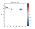
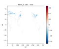
Thus I am not sure whether the discrepancy is due to issues in my python code. Additionally, do you think that QSat_2 is more appropriate for urban canopy cases? Any insights into how RH is computed in CLM for urban area or any tips for reproducing RH would be greatly appreciated! Thanks!
Below is my python code:
I have also attached the original .F90 code below (can't paste it here due to length limitation).
CESM 5.2.015
Have you made any changes to files in the source tree?
No
Describe your problem or question:
I forgot to include RH2M_U in CLM hist output in one of my land-only simulations, thus I want to use PBOT, TSA_U and Q2M_U to derive RH2M_U. I tested the manual calculation on another CLM hist output with both Q2M_U and RH2M_U available.
After checking the CTSM source code (QSatMod.F90, HumanIndexMod.F90, and UrbanFluxesMod.F90), I found two different implementations of the saturation specific humidity calculation:
- QSat(T, p, qs, es, qsdT, esdT) in QSatMod.F90, which is used in UrbanFluxesMod.F90 for calculating RH2M and RH2M_U.
- QSat_2(T_k, p_t, es_mb, de_mbdT, dlnes_mbdT, rs, rsdT, foftk, fdT) in HumanIndexMod.F90, which seems to be used only for diagnostic variables like wet bulb temperature.
- PBOT_U: [50707.625, 106931.5] Pa
- TSA_U: [227.73, 331.94] K (approximately -45.4 to 58.8°C)
- Q2M_U: [4.0e-5, 0.0307] kg/kg
which all seemed to be within valid physical limits and within the coefficient ranges (-75~100°C) used in the polynomial fits.


Thus I am not sure whether the discrepancy is due to issues in my python code. Additionally, do you think that QSat_2 is more appropriate for urban canopy cases? Any insights into how RH is computed in CLM for urban area or any tips for reproducing RH would be greatly appreciated! Thanks!
Below is my python code:
Code:
def Qsat(T_K,p_Pa):
    #water(T>=0°C)
    a=[6.11213476,0.444007856,0.143064234e-01,0.264461437e-03,
    0.305903558e-05,0.196237241e-07,0.892344772e-10,
    -0.373208410e-12,0.209339997e-15]

    #ice(-75°C<=T<0°C)
    c=[6.11123516,0.503109514,0.188369801e-0,0.420547422e-03,
    0.614396778e-05,0.602780717e-07,0.387940929e-09,
    0.149436277e-11,0.262655803e-14]

    T_C=T_K-273.15
    es_hPa=xr.where(
        T_C>=0.0,
        a[0]+T_C*(a[1]+T_C*(a[2]+T_C*(a[3]+T_C*(a[4]+T_C*(a[5]+
        T_C*(a[6]+T_C*(a[7]+T_C*a[8]))))))),
        c[0]+T_C*(c[1]+T_C*(c[2]+T_C*(c[3]+T_C*(c[4]+T_C*(c[5]+
        T_C*(c[6]+T_C*(c[7]+T_C*c[8])))))))
    )
    es_Pa=es_hPa*100
    qs=0.622*es_Pa/(p_Pa-0.378*es_Pa)
    return qs

def QSat_2(T_K, p_Pa):
    lambd_a=3.504
    alpha=17.67
    beta=243.5
    epsilon=0.6220
    es_C=6.112
    vkp=0.2854
    Cf=273.15
    refpres=1000.0

    p_tmb=p_Pa*0.01 # unit:mb
    tcfbdiff=T_K-Cf+beta
    es_mb=es_C*np.exp(alpha*(T_K-Cf)/tcfbdiff)
    ndimpress=(p_tmb/refpres)**vkp
    p0ndplam=refpres*ndimpress**lambd_a
    rs=epsilon*es_mb/(p0ndplam-es_mb)

    return rs

temp_qs_U_Qsat=Qsat(model_TSA_U,model_PBOT)
temp_qs_U_Qsat2=QSat_2(model_TSA_U,model_PBOT)
calc_model_RH2M_U_Qsat=xr.where(model_Q2M_U/temp_qs_U_Qsat*100>100,100,model_Q2M_U/temp_qs_U_Qsat*100) #%
calc_model_RH2M_U_Qsat2=xr.where(model_Q2M_U/temp_qs_U_Qsat2*100>100,100,model_Q2M_U/temp_qs_U_Qsat2*100) #%
I have also attached the original .F90 code below (can't paste it here due to length limitation).

